2009.01.10                                                                                                                 pop_model_2.doc

 

 

An Investigation into the Ancestor/Descendant Paradox

By

John D. Rogers P.Eng

 

 

1.     Introduction. 1

1.1       The Paradox. 1

1.2       Terminology. 1

1.3       Abbreviations and Acronyms. 1

2.     Number of Ancestors. 2

3.     Number of Descendents. 3

4.     Initial Results. 3

4.1       Observations. 6

5.     Modifying the Number of Descendants. 8

5.1       Parents are First Cousins. 8

5.2       Parents are Second Cousins. 8

5.3       Parents are Third Cousins. 8

5.4       Results. 9

6.     Impact of Multiple Cousin Marriages. 11

6.1       Data on the Frequency of Consanguineous Marriages. 11

6.2       Modeling the Consanguineous Marriage Frequency. 12

6.3       Applying the CMF. 13

6.4       Results. 13

6.5       Conclusions. 14

7.     Resolving the Paradox. 15

7.1       Approach. 15

7.2       Looking for a Solution from the Perspective of the Ancestors. 15

7.3       Changing the Consanguineous Marriage Frequency. 17

7.4       Changing the Effect of Consanguineous Marriage Frequency. 17

7.5       Results. 18

8.     Conclusions. 19

 

1.       Introduction

1.1       The Paradox

Doubling the number of ancestors for each previous generation eventually exceeds the number of descendants – this is the ancestor/descendant paradox.

This paper analyzes the growth of an individual’s ancestors and descendants over generations with an objective of investigating and resolving the paradox.

Results and charts used in this paper were obtained using Microsoft Excel spreadsheet pop_model_2.xls.

1.2       Terminology

The following terminology is used in this paper:

Closed	Term for a community (e.g., village or town) where people, in general, do not come in and out. For example, a community that is: owned by one landowner or geologically isolated.
Consanguineous	The union (marriage) of individuals having a common ancestor, e.g., cousins
Cousinship	The relationship of cousins
Crossover	The point in time when the number of descendants equals the number of ancestors
Degree of cousinship	The degree identifies whether the cousin is First, Second, Third, etc.
Marriage	Term used whether parents were married or not
Open	Term for a community (e.g., village or town) where people freely come in and out.

1.3       Abbreviations and Acronyms

The following abbreviations and acronyms are used in this paper:

CM	Consanguineous Marriage
CMF	Consanguineous Marriage Frequency
G	Growth factor
N	Generation number
Y	Year

 

2.       Number of Ancestors

The following table shows how the number of ancestors increases exponentially if it is assumed: each generation is twice the size of the previous; a generation is 25 years; and going back from the year 2000.

 

Gen-eration	Years	Year	Description	Number	Note
0	0	2000	Individual	1
1	25	1975	Parents	2
2	50	1950	Grandparents	4
3	75	1925	Great-grandparents	8
4	100	1900	Great-Great-grandparents	16
5	125	1875	3 x Great-grandparents	32
10	250	1750	8 x Great-grandparents	1024
15	375	1625	13 x Great-grandparents	32,768
20	500	1500	18 x Great-grandparents	1,048,576	@ 1 million
30	750	1250	28 x Great-grandparents	1,073,741,824	@ 1 billion
40	1000	1000	38 x Great-grandparents	1.0995 x 1012	@ 1 trillion
50	1250	750	48 x Great-grandparents	1.1259 x 1015	@ 1 quadrillion
N	25N	2000-25N	(N-2) x Great-grandparents	2N

 

The table shows that using the doubling approach for calculating the number of ancestors soon results in numbers that are greater than the current population of the British Isles (65 million) and the world (7 billion).

3.       Number of Descendents

The approach for calculating the number of descendants assumes the numbers for the first three generations are 1, 2 and 4. From then on it is assumed that the number doubles every 100 years. Therefore there will be 8 descendants by the sixth generation. Again it is assumed that a generation is 25 years. The following table shows these assumptions.

 

 

This approach results in a geometric series of numbers, i.e., each number is multiplied by a growth factor (G) to get the next number. The series (starting at 4) is therefore 4, 4G, 4G², 4G³, 4G⁴ (8).

As 4G⁴ = 8, then . So next number after 4 is 4 x 1.1892 = 4.7568.

Thus the series starts: 1, 2, 4, 4.7568, 5.6569, 6.7272, 8, 9.5137, 11.3137, 13.4543, 16, …..

The starting date for the series (0^th generation) is selected to give a number of descendants in the year that is close to the current population of the British Isles (65 million). Using a starting date of 425 BC gives 56,431,603 descendants after 98 generations.

4.       Initial Results

The following table gives the full results for the numbers of ancestors and descendants calculated using the approaches described in the previous sections.

 

 

Note 1: negative years are BC.

Note 2: The notation 1.23E+12 represents 1,230,000,000,000 (12 places after what was the decimal point).

4.1       Observations

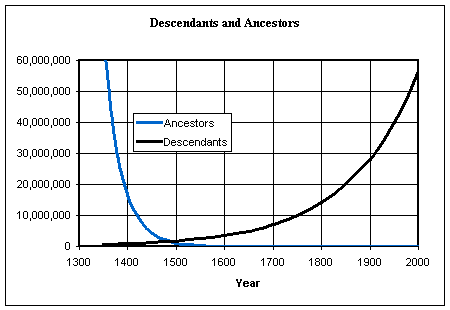
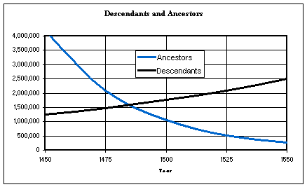
The table shows that the number of descendants is initially low compared with the number of ancestors, but then it rapidly increases. Between 1500 and 1475 AD the number of descendants exceeds the number of ancestors. Thereafter, the number of descendants grows to huge numbers while the number of ancestors steadily decreases.

For the 97^th generation in the year 425 BC, the number of descendants is 158,456,325,028,528,675,187,087,900,672 or 158 octillion.

The following chart shows the number of descendants and ancestors for the years 1300 to 2000 AD.

 

The following chart shows the years 1450 to 1550 AD amplifying the crossover point where the number of descendants exceeds the number of ancestors.

 

 

The crossover point occurs when the number of ancestors equals the number of descendants.

The number of ancestors = 2^N.

The number of descendants = 4.G^(N-2) converting this to use the ancestor generation gives 4.G^(97-N-2)

At crossover 2^N = 4.G^(95-N)

Dividing each side by 4 gives 2^N-2 = G^(95-N)

Taking the logarithm of each side gives (N-2).log 2 = (95-N).log G

N.log 2 – 2.log 2 = 95.log G – N.log G

N (log 2 +log G) = 95.log G + 2 log 2

N =  dividing each side by log G gives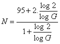

Let, as determined previously,  so

Rearranging gives

Taking the antilogarithms of each side gives  giving[1] k = 4

Substituting the value of k into the formula for N gives

20.6 generations = 20.6 x 25 = 515 years, so the crossover occurred 2000 – 515 years ago in 1485 AD.

5.       Modifying the Number of Descendants

Although doubling the number of descendants for each generation may be valid for recent history, the approach has to be modified so that the number of descendants never exceeds the number of ancestors.

The reason the number of descendants is less than expected is because of inbreeding. The following sections investigate the reduction in ancestors if parents (generation 1) are cousins.

5.1       Parents are First Cousins

First cousins have a common set of grandparents. If first cousins marry they will have 3 sets of grandparents (6 people) instead of 4 sets (8 people). This results in a reduction of ¼ or 25% in the number of descendants.

First cousin marriage is not illegal in the UK. The rate of white first cousin marriages is about 0.5%, however, for other cultures in the UK it is much higher, e.g., 55% for Pakistanis.

5.2       Parents are Second Cousins

Second cousins have a common set of great-grandparents. If second cousins marry they will have 7 sets of great-grandparents (14 people) instead of 8 sets (16 people). This results in a reduction of 1/8 or 12.5% in the number of descendants.

5.3       Parents are Third Cousins

Third cousins have a common set of great-great-grandparents. If third cousins marry they will have 15 sets of great-great grandparents (30 people) instead of 16 sets (32 people). This results in a reduction of 1/16 or 6.25% in the number of descendants.

5.4       Results

The following table shows the numbers of descendants when parents are cousins.

 

Generation	Description	Number if Parents are Unrelated	Number if Parents are Third Cousins	Number if Parents are Second Cousins	Number if Parents are first Cousins
0	Individual	1	1	1	1
1	Parents	2	2	2	2
2	Grandparents	4	4	4	4
3	Great-grandparents	8	8	8	6
4		16	16	14	12
5		32	30	28	24
6		64	60	56	48
7		128	120	112	96
20		1,048,576	1,015,808	983,040	786,432
Reduction		0	6.25%	12.5%	25%

 

By the 20^th generation, if the parents are first cousins there has been a reduction of 262,144 in the number of descendants. This reduction is not all that significant compared with the number if the parents are unrelated. The reduction has only pushed the crossover back from 20.6 generations to 20.9 generations or 7.5 years.

As the degree of the cousinship increases, so the reduction becomes less.

In addition, if the cousins marrying belonged to earlier generations, the reduction is less because then only the previous generations are impacted.

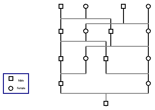
Therefore, there must be multiple consanguineous marriages (CMs). To confirm this, consider the extreme case where all marriages are consanguineous. If both grandfathers are brothers and both grandmothers are sisters then there will 4 great-grandparents instead of the usual 8.  If both great-grandfathers are brothers and both great-grandmothers are sisters then there will 4 great-great-grandparents instead of the usual 16.  In this extreme case, the number of ancestors stabilizes at 4, see the following figure.

 

 

Thus multiple CMs can result in a far reduced number of ancestors. The next section investigates the frequency of these marriages and the resulting number of ancestors.

6.       Impact of Multiple Cousin Marriages

The previous sections showed that if the parents (generation 1) are first cousins, the reduction in descendants was 25%. The following sections investigate the reduction in ancestors if there are multiple marriages between cousins.

6.1       Data on the Frequency of Consanguineous Marriages

The following information applies to the current consanguineous marriage frequency (CMF):

·        the CMF for the UK white population is about 0.5%;

·        the CMF for some immigrant (e.g., Pakistani and Bangladeshi) sections of the UK population is about 55%;

·        the frequency of marriage between second or higher degree cousins is insignificant compared with the frequency of marriage between first cousins in the UK and elsewhere;

·        the CMF[2] for some other countries is:

o       0.2% for the USA,

o       0.6% for Norway,

o       1.5% for Portugal,

o       4.1% for Spain,

o       4.8% for Brazil,

o       5.7% for Japan,

o       39.7% for Jordan, and

o       61.2% for Pakistan;

·        for many countries, the CMF for rural areas is significantly  higher than for urban areas; and

·        it is estimated that 20 percent of all couples worldwide are first cousins.

Data on the historical CMF is very sparse, the following information has been obtained:

·        in the UK, the rate of first cousin marriages was estimated to be:

o       0.32% during the 1920s,

o       1.12% during the 1890s,

o       1.1% from 1775 to 1924 in the ‘open’ parish of Kilmington, and

o       2.25% from 1775 to 1924 in the ‘closed’ parish of Stouton; and

·        it is estimated that 80 percent of all marriages historically have been between first cousins.

6.2       Modeling the Consanguineous Marriage Frequency

The following assumptions are made in order to model the CMF:

·        all CMs are between first cousins;

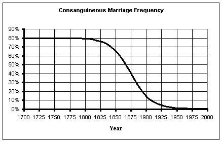
·        prior to the industrial revolution in 1760, the CMF was steady at 80%;

·        the CMF dropped from 1760 to the beginning of the 20^th centenary where it levelled off at 0.5%, this transition was centred around 1875 (Generation 5).

The change in CMF values follows a reverse S-curve. The function which best represents this type of behaviour is the generalized logistic function. This function is modified to fit the above assumptions as follows:

where:

CMF is the consanguineous marriage frequency (%)

L is the lower asymptote = 0.5%

U is the upper asymptote = 80%

G is the growth rate = 0.06 (value selected to fit the data)

Y is the year

The following chart shows the resulting curve of the CMF between 1700 and 1950.

 

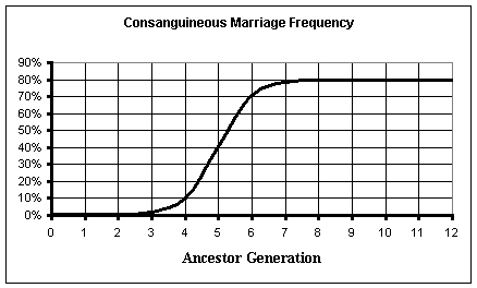
Modifying the above formula to use ancestor generation numbers (gen) instead of years and to start at generation 0 gives:

The following chart shows the resulting curve of the CMF for generations 0 - 12 (2000 – 1700 AD).

 

6.3              Applying the CMF

The CMF is used in calculating the number of descendants for each generation as follows:

·        calculate the number of marriages (half the number of descendants);

·        calculate the CMF for the generation (see above);

·        calculate the number of CMs (multiply the CMF by the number of marriages);

·        calculate the number of descendants in the next generation (reduce the number of descendants in the current generation by the number of CMs and then double).

6.4       Results

The following table shows the results around the generations where crossover occurs. It can be seen that crossover has been pushed back from 1485 (1.6 million ancestors/descendants) to around 960 AD (42,000 ancestors/descendants).

 

 

Although this is an impressive reduction, after crossover, the number of descendants continues to increase by 20% per generation resulting in 1,012,749,142 descendants by the year 425 BC.

Increasing the CMF to 100% stops further growth in the number of descendants, but does not reduce it.

6.5       Conclusions

The results show that even with an 80% CMF, the reductions are still not enough to resolve the paradox.

7.       Resolving the Paradox

7.1       Approach

This section investigates the changes required to resolve the paradox.

7.2       Looking for a Solution from the Perspective of the Ancestors

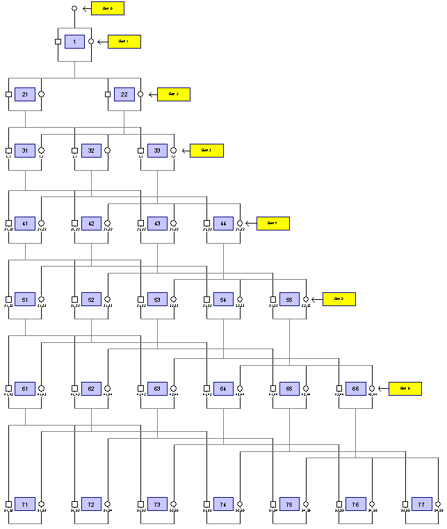
The genealogical chart shows a possible ancestry starting from a single female (Eve) in generation 0. The families are shown in the following chart along with their offspring (B = boy, G = girl). The numbers represent the family numbers of the 4 possible grandparents.

 

Family No	1	2	3	4	5	6	7
1x	BBGG
2x	0, 0 0, 0 BBB	0, 0 0, 0 GGG
3x	1, 1 1, 1 BBB	1, 1 1, 1 GB	1, 1 1, 1 GGG
4x	21, 22 21, 22 BBB	21, 22 21, 22 GB	21, 22 21, 22 GB	21, 22 21, 22 GGG
5x	31, 32 31, 33 BBB	31, 32 31, 33 GB	31, 32 32, 33 GB	31, 33 32, 33 GB	31, 33 32, 33 GGG
6x	41, 42 41, 43 BBB	41, 42 41, 44 GB	41, 42 42, 44 GB	41, 43 43, 44 GB	41, 44 43, 44 GB	42, 44 43, 44 GGG
7x	51, 52 51, 53 BBB	51, 52 51, 54 GB	51, 52 52, 53 GB	51, 53 53, 55 GB	51, 54 54, 55 GB	52, 55 54, 55 GB	53, 55 54, 55 GGG

 

The following table provides a summary.

Generation	Size	Description
0	1	Eve
1	2	Eve has a boy (B) and a girl (G)
2	4	They form 1 family with 2 boys (BB) and 2 girls (GG)
3	6	They form 2 families with offspring BBB and GGG
4	8	They form 3 families with offspring BBB, BG and GGG
5	10	They form 4 families with offspring BBB, BG, BG, BG and GGG
6	12	They form 5 families with offspring BBB, BG, BG, BG, BG and GGG
7	14	They form 6 families with offspring BBB, BG, BG, BG, BG, BG and GGG

 

Observations:

·        it is possible to have a scenario where the previous generations reduce in size instead of increasing because of a high degree of inbreeding:

·        if families have on average:

o       less than 2 children, the population size will reduce,

o       exactly 2 children, the population size will stabilize, and

o       more than 2 children, the population size will increase;

As a result of the above the following changes will be made:

·        the initial population sizes will be 1, 2, 4, 6, 8 and thereafter increase at a rate which doubles every 4 generations: 9, 11, 13, 16, 19, 23, 27, 32 etc.; and

·        the impact of CMs will be increased (see next sections).

7.3       Changing the Consanguineous Marriage Frequency

It is only in recent generations that the population has had the ability to, and has become, much more mobile in the pursuit of jobs, holidays and other entertainment and travel. This increases the probability of marriages outside of the family and the community. Previously, communities became increasingly closed for reasons such as:

·        geographical isolation;

·        lack of transport;

·        religious (Catholics could only marry Catholics);

·        wealthy families wishing to keep their wealth within the family; and

·        mistrust, even hatred of strangers and other communities.

All of the above results in increased inbreeding causing reductions in the number of ancestors. Therefore the CMF will eventually increase to unity (100%). This increase will be achieved as shown in the following table.

 

 

7.4       Changing the Effect of Consanguineous Marriage Frequency

The effect of a first cousin marriage is to reduce the number of grandparents by 2. As the CMF reaches 100% the number of ancestors becomes constant. However as the amount of inbreeding increases, more complex cousinships occur. For example for a pair of grandparents:

·        the two grandfathers my be first cousins as well as third cousins;

·        the two grandmothers my be second cousins;

·        one grandfather may be a second cousin of the other grandmother;

Instead of doubling the number of ancestors for each generation, the above all act to reduce the number of ancestors. Further reductions occur for situations when a man marries a second wife (or visa versa), when a family has multiple children all marrying within the family tree and when more distant cousins are taken into account.

To reflect the increased effect of CMs, a factor k is introduced so that instead of reducing the number of grandparents by 2 it will be reduced by 2(1 + k). Values of k are set as shown in the following table.

 

 

7.5       Results

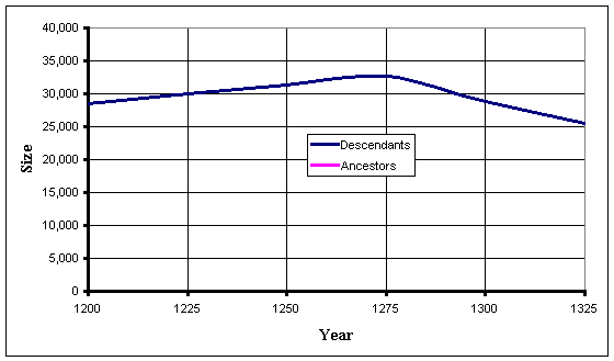
The following chart shows the new results for the years 0 to 2000.

 

 

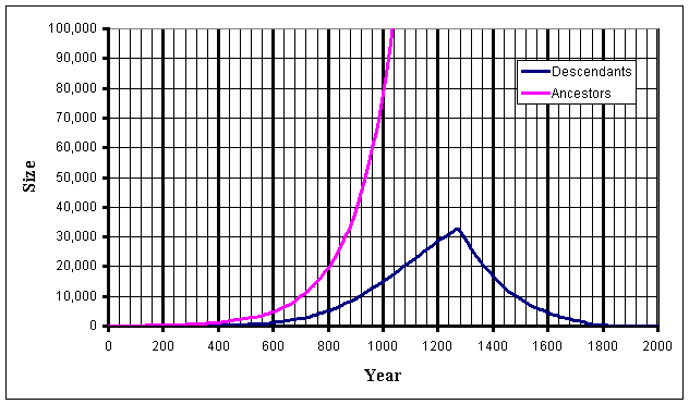
The number of descendants peaks at 32,664 (about 6%) in 1275 AD when the number of ancestors was 524,288. The chart shows the number of descendants increases initially and then peaks following which there appears to be a relatively sharp reduction. However the rate is less than the rate for the descendants and appears less pronounced when the period between 1200 and 1325 AD is shown.

 

 

8.                 Conclusions

This paper has demonstrated the ancestor/descendant paradox and shown that when inbreeding is taken into account the number of descendants eventually reduces thereby refuting the paradox.

Further investigation is required to more precisely quantify the effect of inbreeding, to validate the assumptions made, refine the analysis and to obtain more historical data.